Deep Hebbian Image Encoder
Deep Hebbian Image Encoder
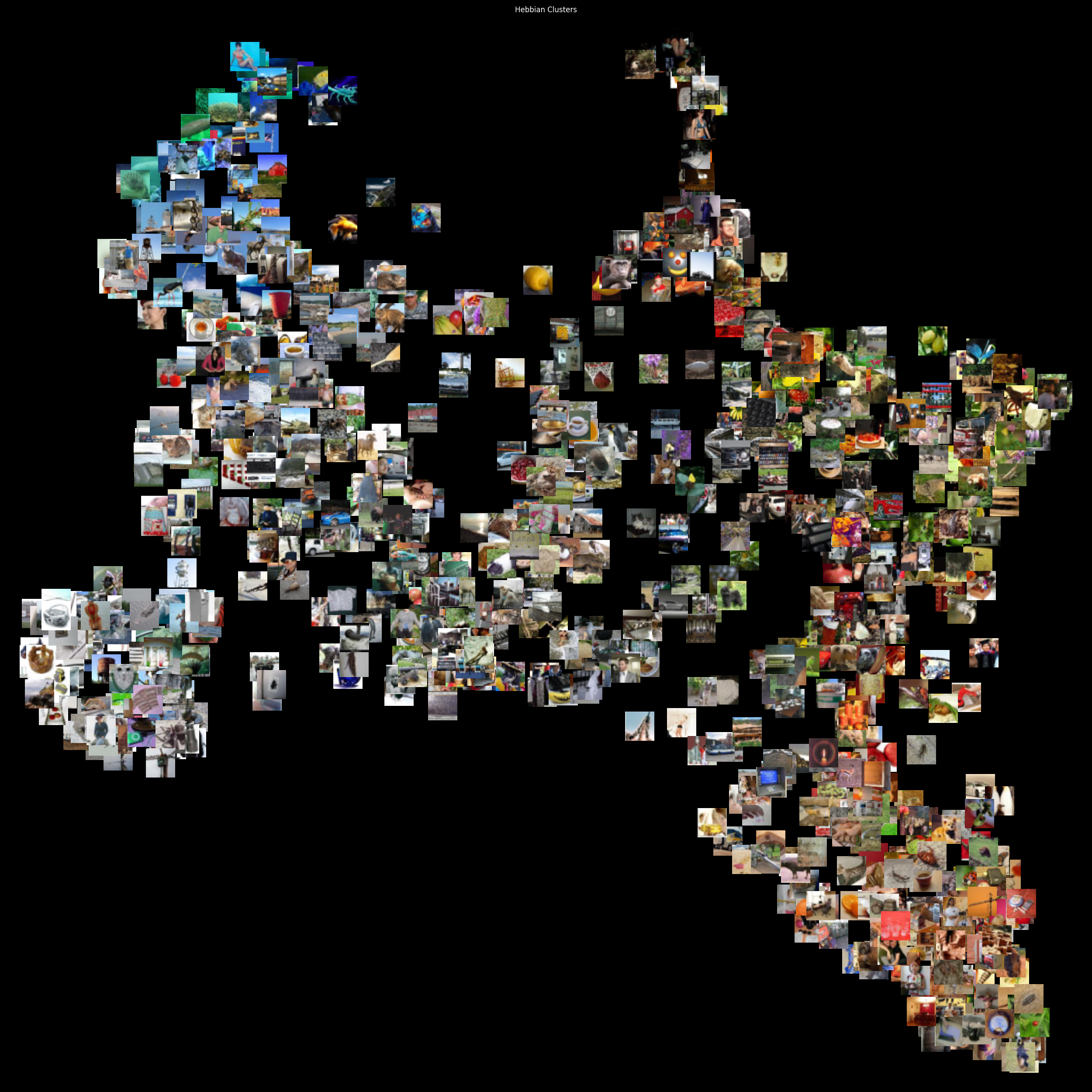
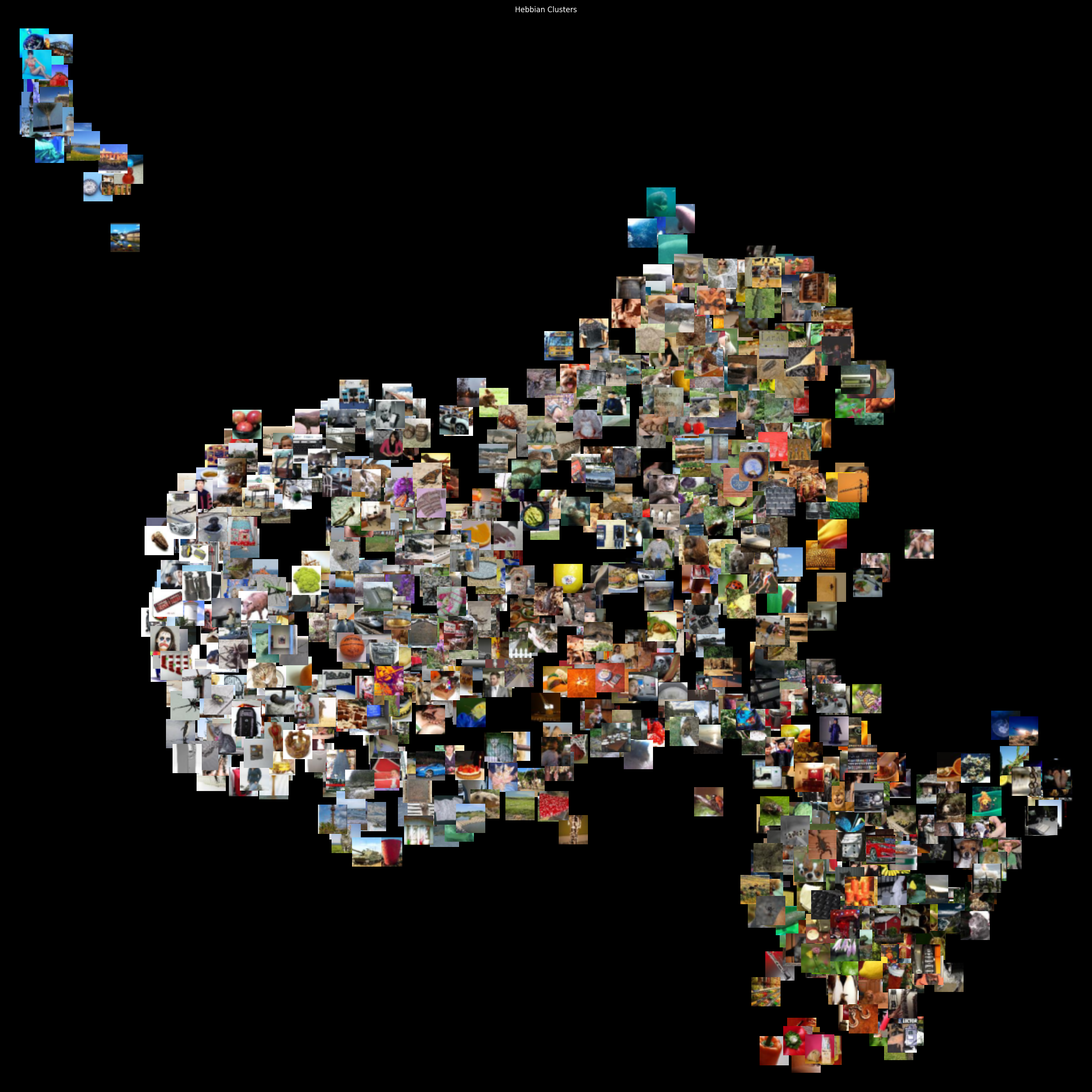
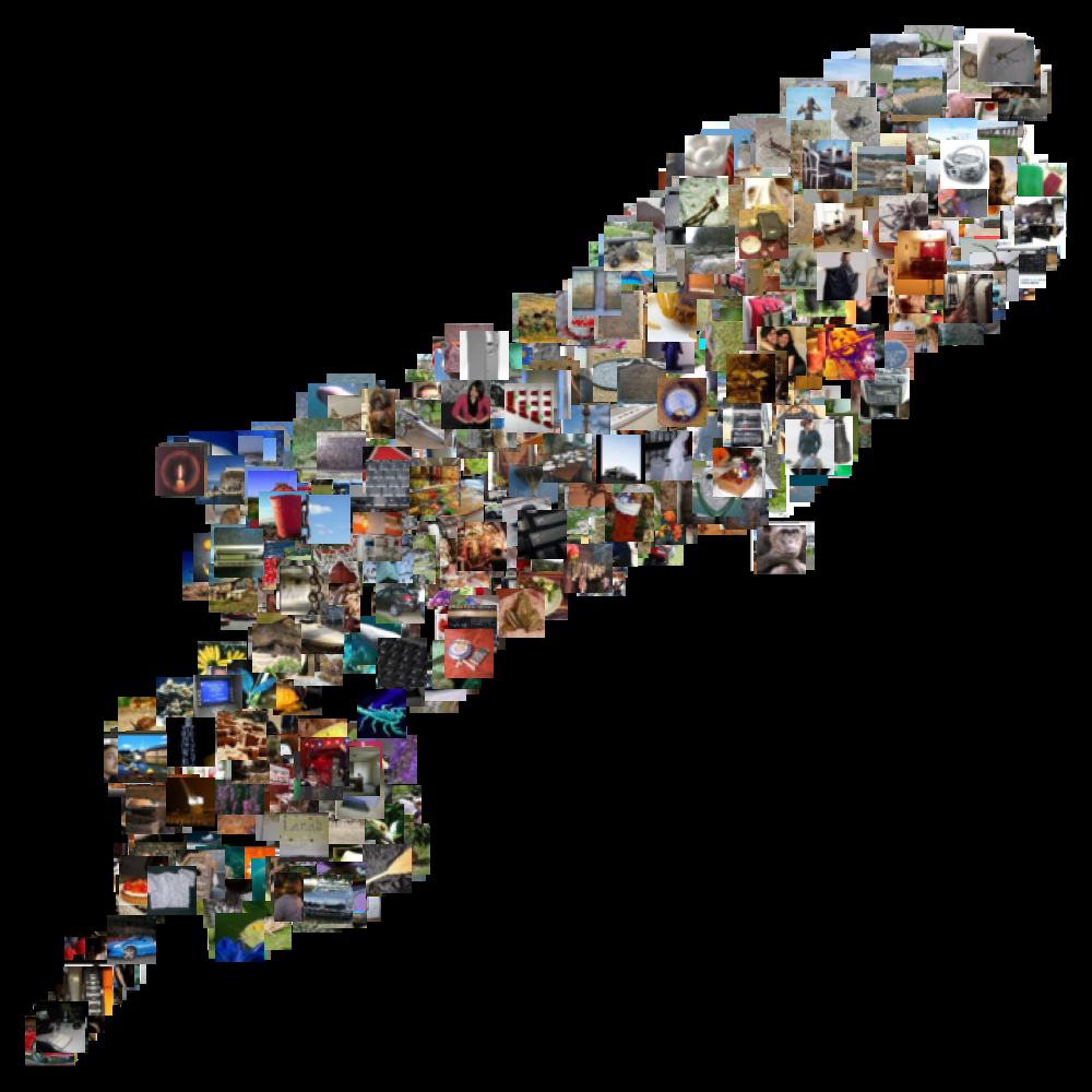
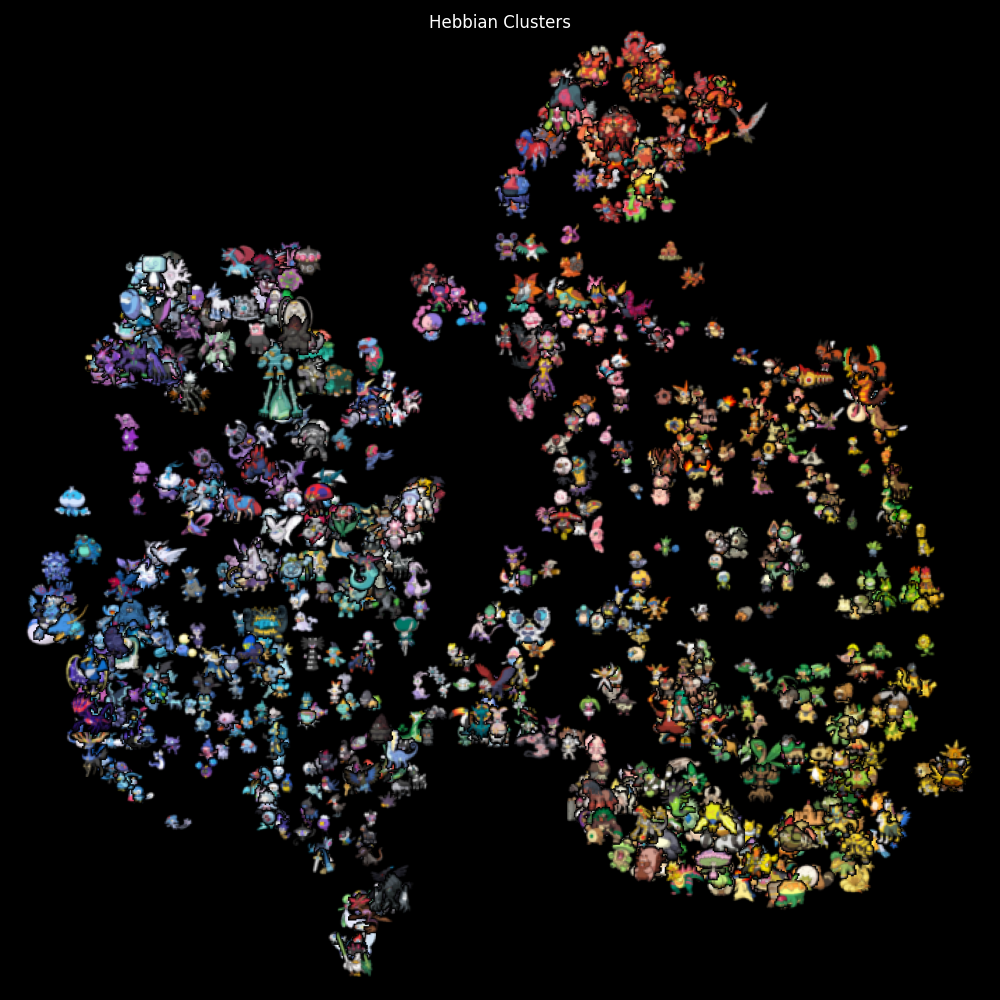
This project explores biologically-inspired Hebbian methods to train stackable image encoders. These models can organize visual information without traditional loss functions or backpropagation. Afterward, the learned image embeddings are visualized using UMAP + K-Means Clustering.
Below is a sample clustering of learned image embeddings from the Tiny ImageNet dataset.
Source code on Github
Why Hebbian? (Biological Analogy)
Unlike traditional neural networks that rely on error signals and gradient descent, Hebbian models operate more like biological brains. There's no supervision, no target output, no error propagation. Just forward input, and strengthening connections between neurons that activate together.
"Neurons that fire together, wire together."
This means the network doesn't know what the correct answer is, it just recognizes and reinforces co-occurrence in the data. If two features appear frequently at the same time, their connection strengthens. Over time, this results in internal representations that reflect the structure of the data, without needing labels or supervision.
This approach mirrors parts of the brain's learning strategy, where connections are locally updated based on experience, rather than global goals. It's simpler, and more biologically plausible, and that simplicity might be useful for efficient or modular systems in the future.
Dataset Preparation
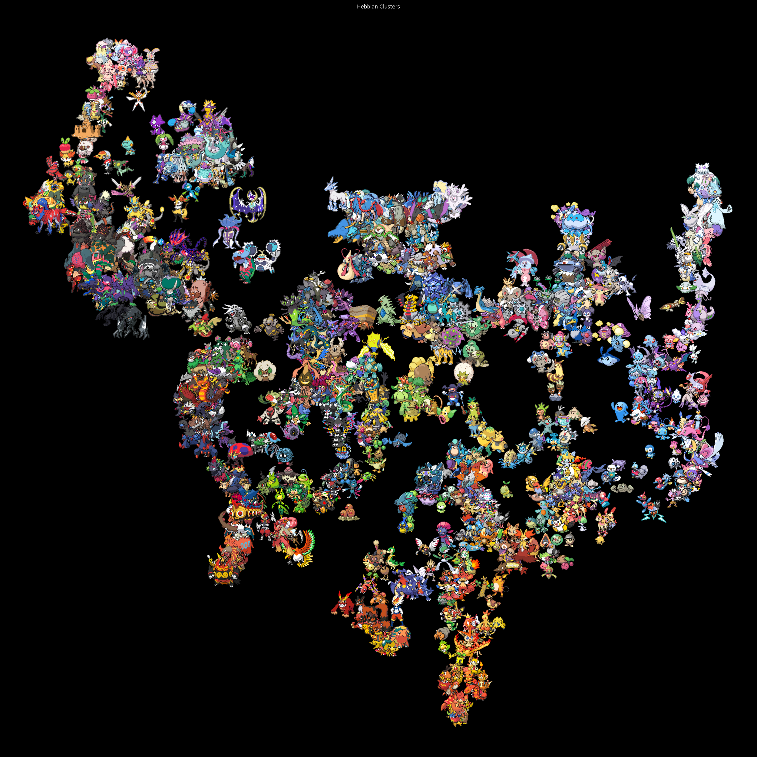
Images are resized to 64×64 for standardization across datasets. For the Pokémon dataset, we extract sprites from a transparent PNG grid:
sprites = load_spritesheet("pokemon_all_transparent.png", sprite_size=(64, 64), tile_size=(96, 96))
For Tiny ImageNet:
dataset = ImageFolder("../data/tiny_imagenet/train", transform=transforms.Compose([
    transforms.Resize((64, 64)),
    transforms.ToTensor()
]))
Hebbian Encoder Architecture
Each Hebbian encoder layer applies:
- A %%3 \times 3%% convolution with stride 2
- ReLU activation
- L2 normalization over spatial dimensions
- Lateral weights updated by Hebbian rule:
$$ \Delta W_{ij} = \eta \cdot \langle a_i \cdot a_j \rangle $$
Where:
- %%\Delta W_{ij}%% is the change in weight from unit %%j%% to %%i%%
- %%\eta%% is the learning rate
- %%a_i%% and %%a_j%% are the activations of units %%i%% and %%j%% respectively
- %%\langle a_i \cdot a_j \rangle%% denotes the batch-averaged outer product
This update promotes co-activation patterns. Inhibition is enforced by subtracting mean activation:
hebbian = torch.einsum("bni,bnj->nij", act_flat, act_flat)  # outer product over batch
delta = 0.001 * hebbian.mean(dim=0)
self.lateral_weights.data += delta.clamp(-1.0, 1.0)
Overall Network Architecture
Input Image (64×64×3/4)
       │
       ▼
┌─────────────────┐    Layer 1: 3/4→16 channels, 64×64→32×32
│  HebbianLayer1  │
│   Conv + Hebb   │    ┌─ Conv2d(3/4→16, k=3, s=2)
│                 │    ├─ ReLU + L2 Norm
│  [32×32×16]     │    ├─ Lateral Connections (16×1024×1024)
└─────────────────┘    └─ Mean Subtraction (Inhibition)
       │
       ▼
┌─────────────────┐    Layer 2: 16→32 channels, 32×32→16×16
│  HebbianLayer2  │
│   Conv + Hebb   │    ├─ Lateral Connections (32×256×256)
│  [16×16×32]     │
└─────────────────┘
       │
       ▼
┌─────────────────┐    Layer 3: 32→64 channels, 16×16→8×8
│  HebbianLayer3  │
│   Conv + Hebb   │    ├─ Lateral Connections (64×64×64)
│   [8×8×64]      │
└─────────────────┘
       │
       ▼
┌─────────────────┐    Layer 4: 64→128 channels, 8×8→4×4
│  HebbianLayer4  │
│   Conv + Hebb   │    ├─ Lateral Connections (128×16×16)
│   [4×4×128]     │
└─────────────────┘
       │
       ▼
    Flatten
  [2048 features]
       │
       ▼
┌─────────────────┐
│  UMAP Reduce    │ ──► 2D Visualization
│   2048 → 2D     │
└─────────────────┘
Spatial-Aware Lateral Connections Explained
Single Channel Spatial Layout:
Original 4×4 feature map:          Flattened to 16 positions:
┌─────┬─────┬─────┬─────┐         ┌─────────────────────┐
│ a₀  │ a₁  │ a₂  │ a₃  │         │ a₀ a₁ a₂ a₃ a₄ ...  │
├─────┼─────┼─────┼─────┤   ────► │                     │
│ a₄  │ a₅  │ a₆  │ a₇  │         │ ... a₁₂ a₁₃ a₁₄ a₁₅ │
├─────┼─────┼─────┼─────┤         └─────────────────────┘
│ a₈  │ a₉  │ a₁₀ │ a₁₁ │
├─────┼─────┼─────┼─────┤
│ a₁₂ │ a₁₃ │ a₁₄ │ a₁₅ │
└─────┴─────┴─────┴─────┘
Lateral Weight Matrix (16×16 for this channel):
     a₀  a₁  a₂  a₃  a₄  a₅  a₆  a₇  a₈  a₉  a₁₀ a₁₁ a₁₂ a₁₃ a₁₄ a₁₅
a₀  │w₀₀ w₀₁ w₀₂ w₀₃ w₀₄ w₀₅ w₀₆ w₀₇ w₀₈ w₀₉ w₀₁₀w₀₁₁w₀₁₂w₀₁₃w₀₁₄w₀₁₅│
a₁  │w₁₀ w₁₁ w₁₂ w₁₃ w₁₄ w₁₅ w₁₆ w₁₇ w₁₈ w₁₉ w₁₁₀w₁₁₁w₁₁₂w₁₁₃w₁₁₄w₁₁₅│
a₂  │w₂₀ w₂₁ w₂₂ w₂₃ w₂₄ w₂₅ w₂₆ w₂₇ w₂₈ w₂₉ w₂₁₀w₂₁₁w₂₁₂w₂₁₃w₂₁₄w₂₁₅│
... │...                                                              │
a₁₅ │w₁₅₀w₁₅₁w₁₅₂w₁₅₃w₁₅₄w₁₅₅w₁₅₆w₁₅₇w₁₅₈w₁₅₉w₁₅₁₀w₁₅₁₁w₁₅₁₂w₁₅₁₃w₁₅₁₄w₁₅₁₅│
Each position can influence every other position in the same channel.
Without Lateral Connections:
┌───┐ ┌───┐ ┌───┐ ┌───┐
│ a │ │ b │ │ c │ │ d │  ← Independent activations
└───┘ └───┘ └───┘ └───┘    No communication between positions
With Lateral Connections:
┌───┐ ┌───┐ ┌───┐ ┌───┐
│ a │↔│ b │↔│ c │↔│ d │  ← Positions influence each other
└─┬─┘ └─┬─┘ └─┬─┘ └─┬─┘
  ↕     ↕     ↕     ↕      Creates spatial competition
┌─┴─┐ ┌─┴─┐ ┌─┴─┐ ┌─┴─┐    and cooperation patterns
│ e │ │ f │ │ g │ │ h │
└───┘ └───┘ └───┘ └───┘
Multi-Channel Lateral Structure
For a layer with C channels and H×W spatial dimensions:
Channel 0: [H×W positions] ──► [N×N lateral weights]
Channel 1: [H×W positions] ──► [N×N lateral weights]
Channel 2: [H×W positions] ──► [N×N lateral weights]
...
Channel C: [H×W positions] ──► [N×N lateral weights]

where N = H × W

Total lateral weights: C × N × N
Example for 32×32→16×16 layer (32 channels):
self.lateral_weights.shape = [32, 256, 256]
                             ↑    ↑    ↑
                             │    │    └─ 256 "to" positions
                             │    └────── 256 "from" positions
                             └─────────── 32 independent channels
Hebbian Learning Step-by-Step
Step 1: Forward Pass
Input Batch: [B, C, H, W]
     │
     ▼ Conv2d + ReLU
Activations: [B, C, H', W']
     │
     ▼ L2 Normalize
Normalized: [B, C, H', W'] (unit norm per spatial map)
Step 2: Flatten for Lateral Processing
act_flat = activations.view(B, C, H'×W')
Result shape: [B, C, N] where N = H'×W'
Step 3: Hebbian Update (No Gradients!)
# Compute outer product for each spatial position
hebbian = torch.einsum("bni,bnj->nij", act_flat, act_flat)
#                       ↑     ↑     ↑
#                       │     │     └─ Output: [N, N] per batch
#                       │     └─────── j-th position activation
#                       └─────────────── i-th position activation

# Average across batch and update weights
delta = 0.001 * hebbian.mean(dim=0)  # [N, N]
self.lateral_weights.data += delta   # Update each channel separately
Step 4: Apply Lateral Connections
# Matrix multiply: activations × lateral weights
lateral = torch.einsum("bci,cij->bcj", act_flat, self.lateral_weights)
#                      ↑     ↑     ↑
#                      │     │     └─ Output activations per channel
#                      │     └─────── Channel-specific weights [N×N]
#                      └─────────────── Input activations [C×N]
Step 5: Inhibition (Competition)
lateral = lateral - lateral.mean(dim=(2,3), keepdim=True)
# Subtract mean → winner-take-all dynamics
Energy, Delta, Norm Logging
During training, the following values are logged per step:
- Energy: mean squared activation across all units, i.e., %%\mathbb{E}[|a|^2]%%
- Delta: mean absolute change in lateral weights
- Norm: Frobenius norm of the lateral weight matrix, i.e., %%|W|_F%%
Example:
[LOG] Step 122: energy=0.1466, delta=0.000166, norm=155.7744
This gives insight into encoder dynamics: stable energy and delta values indicate convergence, while growing norm may suggest over-association.
Feature Extraction
Images are passed through a multi-layer encoder consisting of 4 HebbianEncoder layers. The final feature map is flattened to a 1D vector and stored.
features = model(images)
features = F.normalize(features, dim=1).cpu().numpy()
Hebbian Network Structure
The Hebbian encoder processes 64×64 images using a stack of convolutional layers with stride 2. Each layer halves the spatial resolution while increasing the channel count. Each Hebbian layer also includes lateral recurrent weights trained with Hebbian updates to reinforce co-activation patterns.
# For RGB images (Tiny ImageNet)
model = MultiLayerHebbian([
    (3, 16, (32, 32)),
    (16, 32, (16, 16)),
    (32, 64, (8, 8)),
    (64, 128, (4, 4))
])

# For RGBA images (Pokémon sprites)
model = MultiLayerHebbian([
    (4, 16, (32, 32)),
    (16, 32, (16, 16)),
    (32, 64, (8, 8)),
    (64, 128, (4, 4))
])
Each tuple in the list specifies the parameters for a HebbianEncoder layer:
(in_channels, out_channels, spatial_shape)
This configuration maps as follows:
| Layer | Input Channels | Output Channels | Input Spatial Size | Output Spatial Size |
|---|---|---|---|---|
| 1 | 3/4 (RGB/RGBA) | 16 | 64×64 | 32×32 |
| 2 | 16 | 32 | 32×32 | 16×16 |
| 3 | 32 | 64 | 16×16 | 8×8 |
| 4 | 64 | 128 | 8×8 | 4×4 |
This structure results in a final feature tensor of shape (B, 128, 4, 4) per image, which is flattened to (B, 2048) and used for clustering and visualization.
The spatial argument in each HebbianEncoder is required to initialize the lateral weight matrix:
self.lateral_weights = torch.nn.Parameter(torch.zeros(C, N, N))
where N = H × W (the number of spatial positions per channel). These weights are updated using Hebbian learning:
$$ \Delta W_{ij} = \eta \cdot \langle a_i \cdot a_j \rangle $$
which in code becomes:
hebbian = torch.einsum("bni,bnj->nij", act_flat, act_flat)
delta = 0.001 * hebbian.mean(dim=0)
self.lateral_weights.data += delta
This configuration balances spatial compression and representational capacity, while the Hebbian lateral updates encourage neurons to specialize by detecting and reinforcing co-activation patterns.
Embedding and Clustering Visualization
UMAP is used to project feature vectors to 2D.
reducer = UMAP(n_components=2, random_state=42)
reduced = reducer.fit_transform(features)
Optionally, KMeans clustering is applied to the feature space:
kmeans = KMeans(n_clusters=6, random_state=42).fit(features)
These steps are primarily for visualization and evaluation. They allow us to inspect whether the encoder has organized inputs meaningfully—not as a training objective.
Layout and Plotting
Projected coordinates are normalized to fit inside a square canvas (e.g., 2500x2500 pixels). Margin padding ensures images are not clipped.
reduced -= reduced.min(axis=0)
reduced /= (reduced.max(axis=0) + 1e-8)
reduced *= (canvas_size - 2 * margin)
reduced += margin
Sprites are drawn onto the canvas using their corresponding (x, y) UMAP coordinates.
for (x, y), img in zip(reduced, sprites):
    pil = transforms.ToPILImage()(img).resize((sprite_size, sprite_size))
    canvas.paste(pil, (int(x), int(y)), mask=pil if has_alpha else None)
Code + Results
Tiny ImageNet (Hebbian)
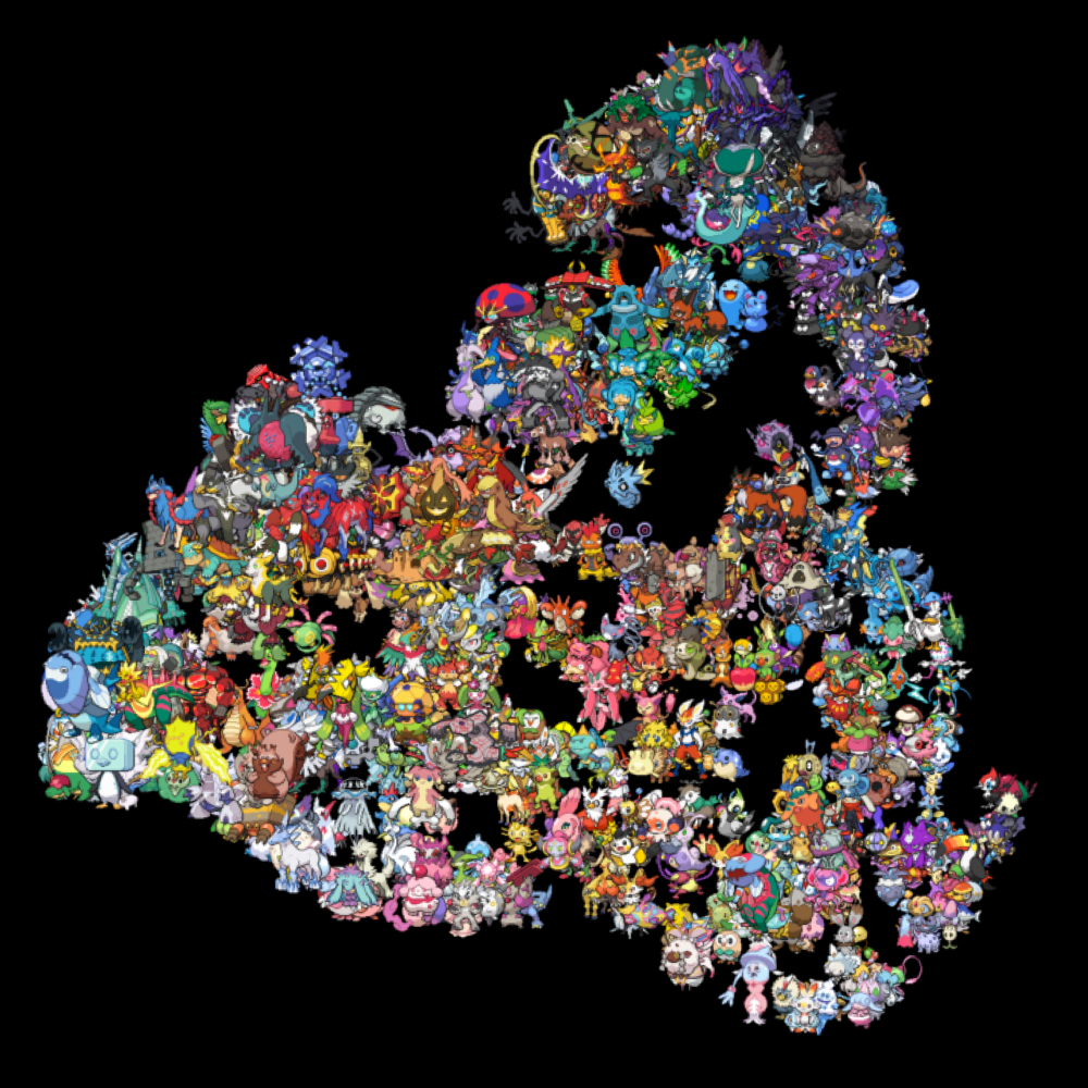
Pokémon Full RGBA Hebbian
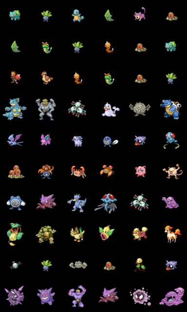
Pokémon Similarity
The first column contains randomly selected Pokémon, and then the most-similar 5 Pokémon are listed to the right.
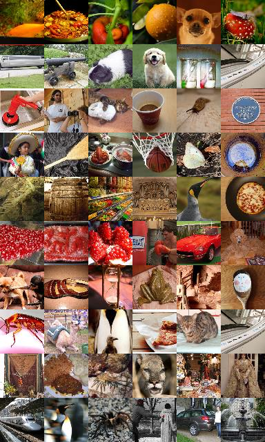
Hebbian Image Encoder (Single-Layer)
This was the first prototype. The first column contains randomly selected image (from Tiny Imagenet), and then the most-similar 5 images are listed to the right.
Hebbian Deep Image Encoder - Tiny ImageNet - Source Code
import sys
import os
import torch
import torch.nn.functional as F
from torch.utils.data import DataLoader
from torchvision import transforms
from torchvision.datasets import ImageFolder
from PIL import Image
import matplotlib.pyplot as plt
import numpy as np
from sklearn.cluster import KMeans
from umap import UMAP

# === Config ===
IMAGE_DIR = "../data/tiny_imagenet/train"
SPRITE_SIZE = (64, 64)
BATCH_SIZE = 8
NUM_IMAGES = 1000
EPOCHS = 50
CLUSTERS = 4
EMBED_SIZE = 32  # thumbnail size
CANVAS_SIZE = 2500

# === Hebbian Network ===
class HebbianEncoder(torch.nn.Module):
    def __init__(self, in_channels, out_channels, spatial):
        super().__init__()
        self.encode = torch.nn.Conv2d(in_channels, out_channels, kernel_size=3, stride=2, padding=1)
        C = out_channels
        N = spatial[0] * spatial[1]
        self.lateral_weights = torch.nn.Parameter(torch.zeros(C, N, N))

    def forward(self, x, step=None):
        act = F.relu(self.encode(x))
        act = act / (act.norm(dim=(2, 3), keepdim=True) + 1e-6)
        B, C, H, W = act.shape
        act_flat = act.view(B, C, -1)

        with torch.no_grad():
            hebbian = torch.einsum("bni,bnj->nij", act_flat, act_flat)
            delta = 0.001 * hebbian.mean(dim=0)
            self.lateral_weights.data += delta
            self.lateral_weights.data.clamp_(-1.0, 1.0)

        lateral = torch.einsum("bci,cij->bcj", act_flat, self.lateral_weights)
        lateral = lateral.view(B, C, H, W)
        lateral = lateral - lateral.mean(dim=(2, 3), keepdim=True)
        act += lateral

        if step is not None:
            print(f"[LOG] Step {step}: energy={act.pow(2).mean():.4f}, delta={delta.abs().mean():.6f}, norm={self.lateral_weights.data.norm():.4f}")

        return act

class MultiLayerHebbian(torch.nn.Module):
    def __init__(self, layer_shapes):
        super().__init__()
        self.layers = torch.nn.ModuleList([
            HebbianEncoder(in_c, out_c, spatial) for (in_c, out_c, spatial) in layer_shapes
        ])

    def forward(self, x, step=None):
        for i, layer in enumerate(self.layers):
            x = layer(x, step=step if i == len(self.layers) - 1 else None)
        return x.view(x.size(0), -1).detach()

# === Load Dataset ===
def load_dataset():
    transform = transforms.Compose([
        transforms.Resize(SPRITE_SIZE),
        transforms.ToTensor()
    ])
    dataset = ImageFolder(IMAGE_DIR, transform=transform)
    subset = torch.utils.data.Subset(dataset, list(range(min(NUM_IMAGES, len(dataset)))))
    loader = DataLoader(subset, batch_size=BATCH_SIZE, shuffle=False)
    return subset, loader

# === Plot Utility ===
def plot_with_images(embeddings, images, title="Hebbian Clusters", size=32, canvas_size=2500):
    fig, ax = plt.subplots(figsize=(canvas_size / 100, canvas_size / 100), facecolor='black', dpi=100)
    ax.set_facecolor('black')
    ax.set_title(title, color='white')
    ax.set_xticks([])
    ax.set_yticks([])

    from matplotlib.offsetbox import OffsetImage, AnnotationBbox

    # Normalize coordinates to canvas
    margin = size * 2
    embeddings -= embeddings.min(axis=0)
    embeddings /= (embeddings.max(axis=0) + 1e-8)
    embeddings *= (canvas_size - 2 * margin)
    embeddings += margin

    for (x, y), img_tensor in zip(embeddings, images):
        img = transforms.ToPILImage()(img_tensor).resize((size, size), resample=Image.BILINEAR).convert("RGB")
        imbox = OffsetImage(img, zoom=1.5)  # zoom factor for visibility
        ab = AnnotationBbox(imbox, (x, y), frameon=False)
        ax.add_artist(ab)

    ax.set_xlim(0, canvas_size)
    ax.set_ylim(0, canvas_size)
    ax.invert_yaxis()
    plt.tight_layout()
    plt.savefig("tinyimagenet_hebbian_cluster_plot.png", facecolor='black')
    print("[SAVED] tinyimagenet_hebbian_cluster_plot.png")

# === Main ===
if __name__ == "__main__":
    dataset, dataloader = load_dataset()
    model = MultiLayerHebbian([
        (3, 16, (32, 32)),
        (16, 32, (16, 16)),
        (32, 64, (8, 8)),
        (64, 128, (4, 4))
    ])

    all_features = []
    for epoch in range(EPOCHS):
        for step, (batch, _) in enumerate(dataloader):
            z = model(batch, step=step) if epoch == EPOCHS - 1 else model(batch)
            if epoch == EPOCHS - 1:
                all_features.append(z)

    features = torch.cat(all_features, dim=0).cpu().numpy()
    features = np.nan_to_num(features)
    features /= (np.linalg.norm(features, axis=1, keepdims=True) + 1e-6)

    reducer = UMAP(n_components=2, random_state=42) #, min_dist=0.2)
    reduced = reducer.fit_transform(features)

    margin = EMBED_SIZE // 2
    reduced -= reduced.min(axis=0)
    reduced /= (reduced.max(axis=0) + 1e-8)
    reduced *= (CANVAS_SIZE - 2 * margin)
    reduced += margin

    all_images = [img for img, _ in dataset]
    plot_with_images(reduced, all_images)
 Arrived
 Ninja Turdle
 Twitch