Genetic Algorithm to Draw Images

Draw Images via genetic programming. The code can all be found on GitHub: here

The Algorithms

There are two algorithms used in Genetic Draw. Both algorithms demonstrate the use of Genetic Programing to evolve an image from DNA(s).

The DNA is a list of genes where each gene encodes a polygon. The polygon could be a square, circle, rectangle, ellipse, triangle, or N-vertex polygon. In addition each gene encodes the color, location (including z-index), transparency, and size of each polygon.

When a specific DNA is "expressed" I iterate over each of the genes and render the encoded polygons to an image. I do this for each of the DNAs. The rendered image is then compared to a target image. The difference between the target image and the actual image is defined as the fitness of the DNA. In this program, 0 is perfect, meaning the evolved image is exactly the same as the target image. This is more accurately defined as the error function and works just as well.

Single Parent Genetic Programming (SingleParentGeneticDraw.kt)

1. Randomly generate a parent DNA.
2. Make a clone of the parent DNA, randomly mutating some of it's genes. We'll call this the child DNA.
3. Measure the fitness of the child DNA. This is done by drawing the polygons to an image and comparing it pixel-by-pixel to a target image.
4. If the child's DNA is more fit than it's parent's DNA, then set the parent to be the child. (The parent is now irrelevant.)
5. Repeat form step 2.

Population-Based Two Parent Genetic Programming (PopulationBasedGeneticDraw.kt)

1. Randomly generate a population of DNAs.
2. Measure the fitness of all of the DNAs and sort them by fitness.
3. Optionally, allowing elitism, select the most fit to succeed to the next generation.
4. Optionally, kill off the bottom x% (lowest fitness) of the population.
5. Using tournament selection or stochastic acceptance determine which remaining DNAs should reproduce to make the next generation of DNAs. Reproduce enough children to repopulate the next generation.
6. After selecting which DNAs to reproduce, via crossover, select 50% of the genes from each parent, apply random mutations to generate children DNAs. The children now become the current population.
7. Repeat form step 2.

Select Renderings & Stats

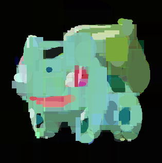
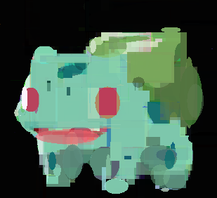
Two versions of Bulbasaur partially evolved. Used sexual reproduction via two parents. Population used stochastic acceptance with elitism to generate next populations.

Two GIFs showing the evolution of a square.

GIF showing the evolution of the DataRank and Simply Measured logos.

Evolutions of Mario. The first is using a polygon rendering DNA. The second and third are using DNAs that render fixed position/sized pixels of size 4x4px and 8x8px.

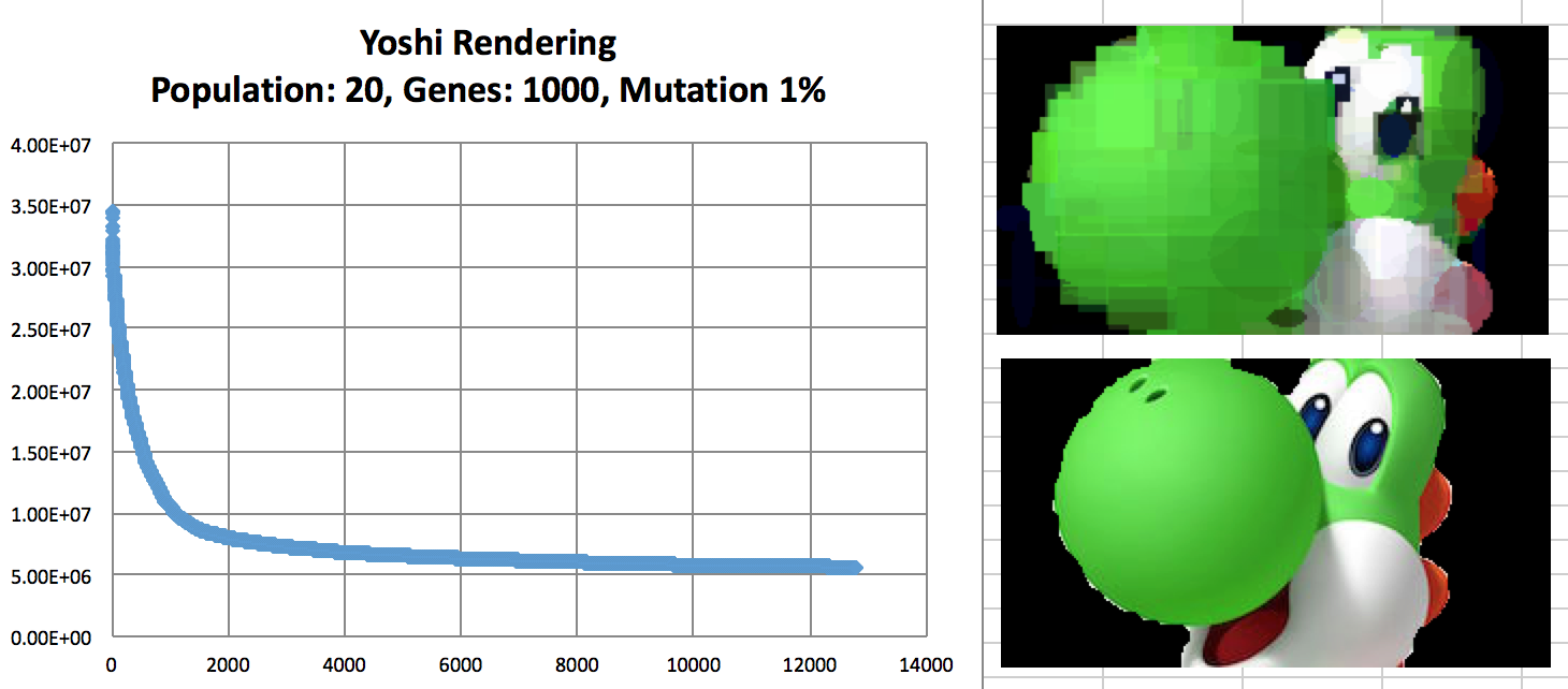
Evolution of Yoshi with convergence rate.

Adding alpha channels to the polygons results in a considerable performance drop (about 7x). While adding alpha results in better results, there are options to remove the alpha channel. Below are three renderings, the first two use alpha (left 2500 genes, middle 2000 genes), and the right image demonstrates no transparency.

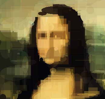
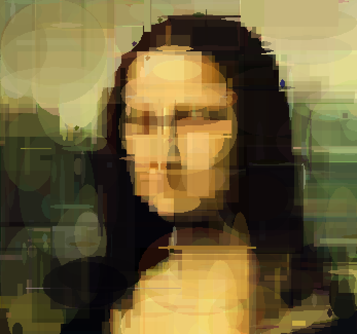
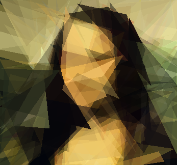
The canonical examples I found on the internet seem to be the evolution of Mona Lisa. Most examples I found demonstrated using triangles. I found that I had better results by mixing many shapes together. On the left is Mona Lisa evolved using rectangles and ellipses. Below, the first two evolutions demonstrate 1000 and 2000 genes containing only rectangles and ellipses, and the third using only triangles.

Mutation Rates and their effect on learning. Not normalized to generation count, you'll have to do some manual comparing. As expected, 10% performs better than 1% and 50%. I did not try a large number of intermittent values. (Note the generation count to see the faster convergence.)

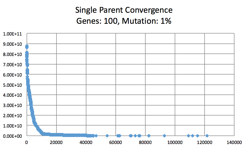
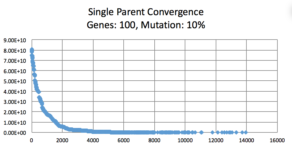
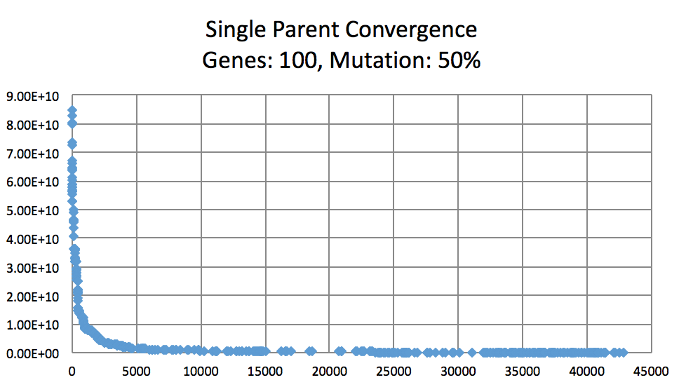
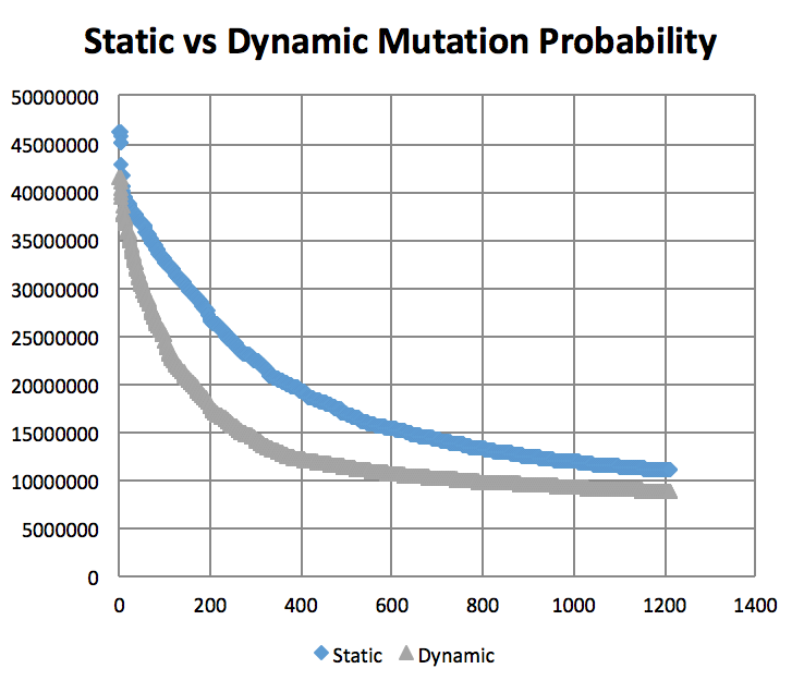
On the topic of mutation, a low mutation rate means that the image converges slowly but gradually. However, there is a caveat. With a low mutation rate the algorithm is less likely to explore new search spaces which may be required to escape from a local minima. Similarly having too large of a mutation rate results in the algorithm constantly making too large of changes which result in a slowed convergence. A large mutation rate may serve well early on in the evolution, however, as time elapses, the required micro changes to finesse the model are less likely to occur. This is analogous to having too high of a learning rate in neural networks. Instead of adopting a simulated annealing-like model with a decreasing mutation rate, I implemented a random bounded mutation rate for each child produced. The results were more successful than a static mutation probability.

Our good friend Kirby, evolved using both pixel and polygon rendering DNAs.

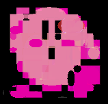
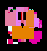
However, one of our Kirby's didn't evolve so well. But why? It turns out that I had a bad fitness function. Specifically my fitness function compared the raw difference between raw RGB integer values between the evolved and target images. That is red is encoded in higher bits than green, and green higher than blue. This means that a difference between reds is significantly larger than differences between greens or blue and thus the genetic algorithm will perceive improvements of red being more important than blue. In other words, I introduced a bias in the fitness function. The result was random blue blotches in many of the renderings.

More of the statistics and graphs can be found in an excel file here.

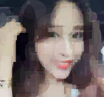
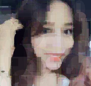
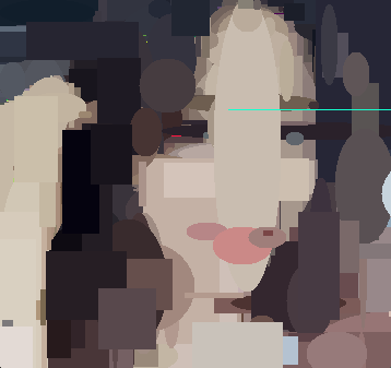
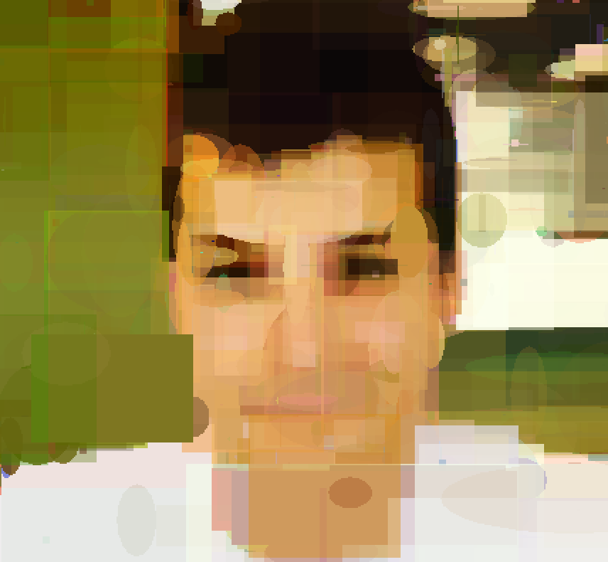
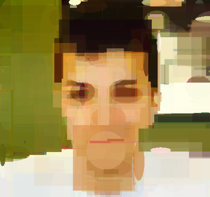
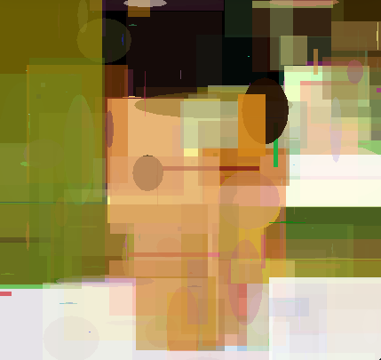
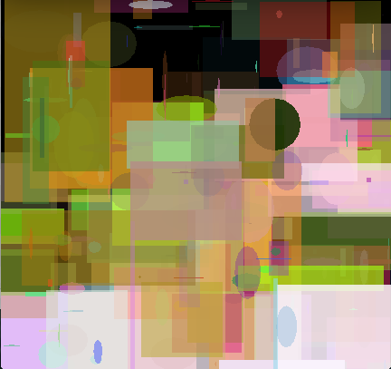
And finally, a current snapshot of my profile being evolved. :)

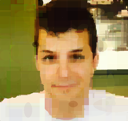
And previous versions.